# Reinforcement Learning Notes: State and Action Values

# 1. State Value / State Value Function

$$v_{\pi}(s) = \mathbb{E}[G_t | S_t = s]$$

• The state value function $v_{\pi}(s)$ represents the expected discounted return when starting in state $s$ and following policy $\pi$.
• Core Concept: Discounted return average upon a given policy.
• Deterministic Scenario: If the policy $\pi(a|s)$, transition probability $p(s'|s, a)$, and reward $p(r|s, a)$ are all deterministic, the State Value is identical to the Return.

# 2. Bellman Equation

The Bellman equation characterizes the relationship among the state-value functions of different states.

# 2.1 Scalar Form

$$v_{\pi}(s) = \sum_{a} \pi(a|s) \left[ \sum_{r} p(r|s, a)r + \gamma \sum_{s'} p(s'|s, a)v_{\pi}(s') \right], \forall s \in S$$

• $\pi(a|s)$ is a given policy, which assigned a probability for action $a$ at state $s$.
• Solving the Bellman equation is called Policy Evaluation.

# 2.2 Matrix-Vector Form

$$v_{\pi} = r_{\pi} + \gamma P_{\pi} v_{\pi}$$

• $v_{\pi} = [v_{\pi}(s_1), \dots, v_{\pi}(s_n)]^T$ is the value function at all states.
• $r_{\pi} = [r_{\pi}(s_1), \dots, r_{\pi}(s_n)]^T$ (Immediate reward under policy $\pi$)
  • Calculation: $r_{\pi}(s) = \sum_{a} \pi(a|s) \sum_{r} p(r|s, a)r$
• $P_{\pi}$: State transition matrix under policy $\pi$.

# 3. Solving State Values (for a certain policy)

State values can be obtained through:

• Direct Solution: $v_{\pi} = (I - \gamma P_{\pi})^{-1} r_{\pi}$
• Iterative Solution: $v_{k+1} = r_{\pi} + \gamma P_{\pi} v_k$, where subscript $k$ represents iterate step.

# 4. Action Value

The action value function $q_{\pi}(s, a)$ is the expected return starting from state $s$, taking action $a$, and following policy $\pi$.

$$q_{\pi}(s, a) = \mathbb{E}[G_t | S_t = s, A_t = a]$$

$$v_{\pi}(s) = \sum_{a} \pi(a|s) q_{\pi}(s, a)$$

$$q_{\pi}(s, a) = \sum_{r} p(r|s, a)r + \gamma \sum_{s'} p(s'|s, a) v_{\pi}(s')$$

• Compare different actions and select the one with the maximum value (Greedy selection).

# Optimal Policy and Iterative Algorithms

# 1. Bellman Optimal Equation

An optimal policy $\pi^*$ is optimal if $v_{\pi^*}(s) \geq v_{\pi}(s)$ for all $s$ and for any other policy $\pi$.

# 1.1 Element-wise Form

For all $s \in S$:

$$v(s) = \max_{\pi} \sum_{a} \pi(a|s) \left[ \sum_{r} p(r|s, a)r + \gamma \sum_{s'} p(s'|s, a)v(s') \right] \\=\max_{\pi} \sum_{a} \pi(a|s) q(s, a)$$

• Given probability or system model: $p(r|s, a), p(s'|s, a)$
• Reward $r$
• Gamma $\gamma$

# 1.2 Matrix-Vector Form

$$v = \max_{\pi} (r_{\pi} + \gamma P_{\pi} v)$$

The optimal solution is a deterministic greedy policy:

• $\pi^*(a|s) = 1$ if $a = a^*$, else $0$.
• $a^* = \text{argmax}_a q(s, a)$.

$$f(v):=\max_{\pi}(r_{\pi}+\gamma P_\pi v)$$

$$v=f(v)$$

where

$$\left[f(v)\right]_s=\max_{\pi}\sum_{a} \pi(a|s)q(s, a), s\in S$$

# 2. Contraction Mapping Theorem

A fixed-point problem: $v = f(v)$.

• Theorem: If $f$ is a contraction mapping

$$||f(x_1) - f(x_2)|| \leq \gamma ||x_1 - x_2||,\text{ where } \gamma\in(0, 1)$$

, then a unique fixed point $x^*$ exists.

• Algorithm: The sequence $x_{k+1} = f(x_k)$ converges to $x^*$, when $k \to \infty$.
• Application: $f(v) = v$ in RL is a contraction mapping fix point problem.

# 3. Value Iteration (VI) Algorithm

$$v_{k+1} = f(v_k) = \max_{\pi} (r_{\pi} + \gamma P_{\pi} v_k)$$

• Step 1 Policy update: $\pi_{k+1} = \text{argmax}_{\pi} (r_{\pi} + \gamma P_{\pi} v_k)$. Use current $v_k$ select action that maximize $q_k(s, a)$
• Step 2: $v_{k+1} = r_{\pi_{k+1}} + \gamma P_{\pi_{k+1}} v_k$.
• Note: $v_k$ is not the true state value of the intermediate policy. Since $v_k$ does not satisfy Bellman equation.
• Step 3: Stop iteration when $v_k$ changes below the threshold.

q-table explicit expression of $q(s, a)$, list all states and actions on a matrix.

# 4. Policy Iteration (PI) Algorithm

• Step 0: Initial random $\pi_0$
• Step 1: Policy Evaluation (PE): Solve

$$v_{\pi_k} = r_{\pi_k} + \gamma P_{\pi_k} v_{\pi_k}.$$

Closed form: $v_{\pi_k} = (I - \gamma P_{\pi_k})^{-1} r_{\pi_k}$
Iterative: $v^{(j+1)} = r + \gamma P v^{(j)}$

• Step 2: Policy Improvement (PI): $\pi_{k+1} = \text{argmax}_{\pi} (r_{\pi} + \gamma P_{\pi} v_{\pi_k})$.

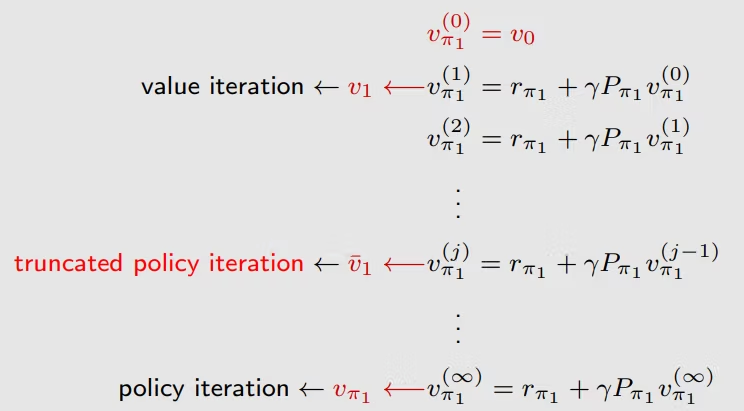
# 5. Comparison: VI and PI

When solving for the value function:

• Value Iteration: Only 1 step of evaluation ($j=1$) before updating $\pi$.
• Truncated PI: $j$ steps of evaluation.
• Policy Iteration: Full evaluation ($j \to \infty$) before updating $\pi$.